The Economic Production Quantity Model
The classical economic production quantity model is presumably one of the most used planning model of all times. Unfortunately, it is often used in situations when its underlying assumptions are not met.
Its assumptions are:
- |
a single product |
- |
stationary demand with constant demand rate over time, $D$ |
- |
finite production rate, $p$ |
- |
setup costs, $s$ |
- |
holding costs, $h$ |
The following figure shows the development of the inventory over two production cycles.
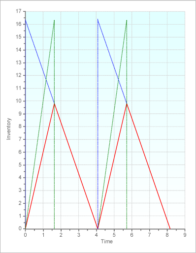
The blue line shows the inventory development that would occur with an infinite production speed. The green line shows the inventory development that would occur without any demand. The red line shows the actual development of the inventory.
In order to find the optimum lot size the first derivative of the the cost function is computed, set to zero and solved for $q$. Let $\rho=\frac{p}{D}$. Then the cost function is the sum of the average setup costs and holding costs per period.
$C(q) = s \cdot \frac{D}{q}+ h \cdot \frac{q}{2} \cdot (1-\rho) $
The first derivative is
$\frac {dC(q)}{dq} = - s \cdot \frac{D}{q^2}+ \frac{h}{2} \cdot (1-\rho) $
Setting this equation equal to zero and solving for $q$ leads to the classical formula for the optimum production quantity:
$q_\mathrm{opt} = \sqrt{\frac{2\cdot s \cdot D}{h\cdot(1-\rho)}}$
This is the exact solution of a clearly defined optimization model. However, for the application of this model in practice it is required that the assumptions of the model are met. If this is not the case, then the optimum production quantity is only a number. A critical point is the development of the demand, which must be stationary. Another point is the availability of the correct setup costs. These should reflect the opportunity costs associated with a setup, e.g. caused by lost setup time. However, the economic value of setup time is usually only known if the optimum lot sizes have been determined. However, if the optimum lot sizes are known, why then use the above model?
If the optimum solution according to the EPQ model is installed in a situation, when multiple products are processed by the same resource in sequence, then the "optimum" lot sizes usually are not feasible. The following example illustrates this situation. Consider seven products with product-specifi data (demand rates, production rates, setup times, setup costs), and holding costs. All products are produced on the same machine. Using the above square root formula for the optimum lot size, we obtain product-specific lot sizes.. If these lot sizes are implemented, the production schedule looks as follows:
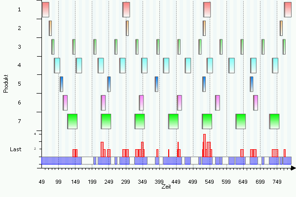
Obviously, this production plan is not feasible, as the resource is overloaded by multiple products simultaneously several times, which can easily be seen from the load chart displayed in the lower part of the graph. Shifting the production of selected products into the future does not solve the problem, as then there will not be enough inventory to fill the demand during the time when a product is not produced. In order to find a feasible production plan, the lot sizes and the production sequence must be computed simultaneously. Several modeling approaches are available for this purpose. One of these models is known as the Economic Lot Scheduling Problem (ELSP).
Note: In industrial practice very often the time is not considered as a continuous variable. By contrast, it is devided into discrete time periods (buckets) with demands that are not constant over time but rather period-specific. In this case the above square root formula is not the solution to the associated optimization problem. In this case, it solves the wrong optimization model, as the inventory shows a dynamic behavior.