Dynamic Lotsizing with Random Demand in an MRP System
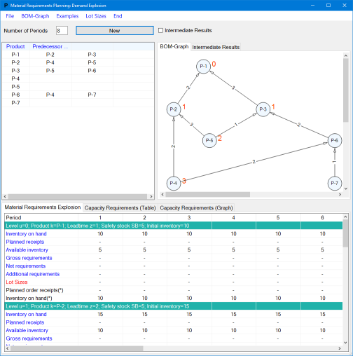
Standard software systems following the MRP (material requirements planning) planning environment perform the calculation of derived demand (demand explosion calculus) based on deterministic demand data. Consider the following example, where the production plan for a selected product is shown. According to the MRP approach, the gross requirements, which are assumed deterministic, have been translated into net requirements which in turn have been combined to production lot sizes.
| Period | 1 | 2 | 3 | 4 | 5 | 6 | 7 | 8 | 9 | 10 |
| Gross requirements | 77 | 42 | 38 | 21 | 26 | 112 | 45 | 14 | 76 | 39 |
| Net requirements | 77 | 42 | 38 | 21 | 26 | 112 | 45 | 14 | 76 | 39 |
| Additional requirements | - | - | - | - | - | - | - | - | - | - |
| Lot sizes | 204 | - | - | - | - | 171 | - | - | 115 | - |
| Planned order receipts(*) | 204 | - | - | - | - | 171 | - | - | 115 | - |
| Inventory on hand(*) | 127 | 85 | 47 | 26 | - | 59 | 14 | - | 39 | - |
If the demand is deterministic, immediately before the production of a new lot the inventory on hand is equal to 0. However, if gross requirements are random, then the risk of backorders exists. Assume that the period demands follow a normal distribution with the above-given gross requirements as expected values and a coefficient of variation (=standard deviation/mean) of 0.3.
For the given production plan, the following development of the system will be observed:
Demand |
Expected |
||||
t |
Mean |
Std.-Dev. |
Lotsize |
Stock on hand |
Backorders |
1 |
77 |
23.1 |
204 |
127 |
0 |
2 |
42 |
12.6 |
0 |
85.0044 |
0.0043 |
3 |
38 |
11.4 |
0 |
47.6076 |
0.6033 |
4 |
21 |
6.3 |
0 |
29.0276 |
2.42 |
5 |
26 |
7.8 |
0 |
12.1193 |
9.0917 |
6 |
112 |
33.6 |
171 |
61.0513 |
2.0513 |
7 |
45 |
13.5 |
0 |
26.6776 |
10.6263 |
8 |
14 |
4.2 |
0 |
18.9307 |
6.2531 |
9 |
76 |
22.8 |
115 |
46.0157 |
6.8955 |
10 |
39 |
11.7 |
0 |
21.5149 |
14.4992 |
The last column shows the backorders that newly occurred in each period. Over the ten periods the fillrate is 89.37%. In order to reduce the amount of backorders, in the literature and from SCM software vendors it is proposed to include safety stock in the MRP calculations. In this case, the available inventory is reduced by the safety stock which results in an increase of the net requirements. With these changed net demands, the lotsizes are calculated.
Interestingly, most textbooks on Operations Management include a chapter on MRP, but omit the problems associated with uncertainty of demand in this planning environment. Moreover, SCM (APS, MRP) software vendor often use false concepts to account for unceratinty.
One proposal is to set the safety stock as a multiple of the average demand. In the above example, the average demand is 49 units. Let's set the safety stock to 49 and observe the behaviour of the system. As at the beginning of the planning horizon there is no inventory available, the net demand increases by 49 to 126. Consequently, the optimum production plan has changed, as the lotsize in period 1 is increased by 49. If the demands were deterministic, then immediately before a replenishment the stock on hand is 49.
| Period | 1 | 2 | 3 | 4 | 5 | 6 | 7 | 8 | 9 | 10 |
| Inventory on hand | - | 49 | 49 | 49 | 49 | 49 | 49 | 49 | 49 | 49 |
| Available inventory | -49 | - | - | - | - | - | - | - | - | - |
| Gross requirements | 77 | 42 | 38 | 21 | 26 | 112 | 45 | 14 | 76 | 39 |
| Net requirements | 126 | 42 | 38 | 21 | 26 | 112 | 45 | 14 | 76 | 39 |
| Additional requirements | - | - | - | - | - | - | - | - | - | - |
| Lot sizes | 253 | - | - | - | - | 171 | - | - | 115 | - |
| Planned order receipts(*) | 253 | - | - | - | - | 171 | - | - | 115 | - |
| Inventory on hand(*) | 176 | 134 | 96 | 75 | 49 | 108 | 63 | 49 | 88 | 49 |
In this case the development of the system is as follows:
Demand |
Expected |
||||
t |
Mean |
Std.-Dev. |
Lotsize |
Stock on hand |
Backorders |
1 |
77 |
23.1 |
253 |
176 |
0 |
2 |
42 |
12.6 |
0 |
134 |
0 |
3 |
38 |
11.4 |
0 |
96.003 |
0.003 |
4 |
21 |
6.3 |
0 |
75.0496 |
0.0466 |
5 |
26 |
7.8 |
0 |
49.6847 |
0.6351 |
6 |
112 |
33.6 |
171 |
108.1292 |
0.1292 |
7 |
45 |
13.5 |
0 |
65.0058 |
1.8766 |
8 |
14 |
4.2 |
0 |
52.714 |
1.7082 |
9 |
76 |
22.8 |
115 |
89.0315 |
1.0282 |
10 |
39 |
11.7 |
0 |
54.3316 |
4.3 |
The overall fillrate is now 98.01%. Which of course is much higher. However, using a multiple of the average demand as a safety stock norm is false, as uncertainty is not associated with the mean demands, but with its variation. If the coefficient of variation of the demand would be, say 0.1, then according to the above stock norm the safety stock would not change. However, the system behaviour would be as follows:
Demand |
Expected |
||||
t |
Mean |
Std.-Dev. |
Lotsize |
Stock on hand |
Backorders |
1 |
77 |
7.7 |
253 |
176 |
0 |
2 |
42 |
4.2 |
0 |
134 |
0 |
3 |
38 |
3.8 |
0 |
96 |
0 |
4 |
21 |
2.1 |
0 |
75 |
0 |
5 |
26 |
2.6 |
0 |
49 |
0 |
6 |
112 |
11.2 |
171 |
108 |
0 |
7 |
45 |
4.5 |
0 |
63.0001 |
0.0001 |
8 |
14 |
1.4 |
0 |
49.0043 |
0.0041 |
9 |
76 |
7.6 |
115 |
88 |
0 |
10 |
39 |
3.9 |
0 |
49.0175 |
0.0175 |
Obviously, with an uncertainty this low, almost no backorders occur and the overall fillrate is 100%. If the fillrate targeted by the management is less than 100%, then inventory levels and holding costs are too high.
Other proposals include the use of methods that basically originate in the stochastic inventory theory developped for the case of stationary demand. These methods are also not appropriate, as they neglect the dynamic character of the (random) demand.
Note that whatever method for calculating an external safety stock is used, the observed fillrate is uncontrollable.
In addition, there is a second problem: it is not taken into consideration that the lot sizes have an impact on the absorption of risk. For example, with large lot sizes, the safety stock required to guarantee a target service level may be zero or even negative. As a consequence, the target service level which should be the basis for the safety stock calculation is met only by chance.
As a systematic planning procedure, a stochastic lotsizing model can be applied when the demand is dynamic and random. Thereby simultaneously randomness and dynamic conditions are considered. In the above example, for a coefficient of variation and a target fillrate of 95% the following production plan would be optimal.
Demand |
Expected |
||||
t |
Mean |
Std.-Dev. |
Lotsize |
Stock on hand |
Backorders |
1 |
77 |
23.1 |
208 |
131.0586 |
0 |
2 |
42 |
12.6 |
0 |
89.0611 |
0.0024 |
3 |
38 |
11.4 |
0 |
51.4885 |
0.4275 |
4 |
21 |
6.3 |
0 |
32.396 |
1.9075 |
5 |
26 |
7.8 |
0 |
14.2566 |
7.8607 |
6 |
112 |
33.6 |
298 |
190.4114 |
0.0001 |
7 |
45 |
13.5 |
0 |
145.425 |
0.0136 |
8 |
14 |
4.2 |
0 |
131.4513 |
0.0263 |
9 |
76 |
22.8 |
0 |
59.3759 |
3.9246 |
10 |
39 |
11.7 |
0 |
30.7091 |
10.3332 |
In the case of a coefficcient of variation of 0.1 we get:
Demand |
Expected |
||||
t |
Mean |
Std.-Dev. |
Lotsize |
Stock on hand |
Backorders |
1 |
77 |
7.7 |
195 |
117.8024 |
0 |
2 |
42 |
4.2 |
0 |
75.8024 |
0 |
3 |
38 |
3.8 |
0 |
37.8025 |
0.0001 |
4 |
21 |
2.1 |
0 |
16.9741 |
0.1717 |
5 |
26 |
2.6 |
0 |
1.0016 |
10.0275 |
6 |
112 |
11.2 |
284 |
162.5589 |
0 |
7 |
45 |
4.5 |
0 |
117.5589 |
0 |
8 |
14 |
1.4 |
0 |
103.5589 |
0 |
9 |
76 |
7.6 |
0 |
27.9961 |
0.4372 |
10 |
39 |
3.9 |
0 |
2.8565 |
13.8604 |
In both cases the production plan is cost-optimal with respect to a given fillrate of 95%.
The above calculations have been performed with the educational software Production Management Trainer.
For more information on inventory Management methods see here.